

The SIGN function takes an input value, and returns either a 1, 0 , or -1, depending on whether or not the value is a positive, zero, or a negative, respectively.
Syntax
= SIGN([number])number = any numerical value, can be hardcoded, a cell reference, or a calculation

Explanation
This function is part of the "Math and Trigonometry" function group. Its purpose is to return a set value (1, 0, -1) depending on the input value fed in, as seen in the table above.
If the input value is non-numerical, a #VALUE error will be returned. All inputs whether a reference or formula, need to be a numerical value and not a string or error.
Examples
1. Using the SIGN function to Identify Positive and Negative Numbers
This is the most basic use of the SIGN function. By feeding in one input, the function will return a 1 if the value is positive, 0 if the value is a 0, and a -1 if the value is negative.
It is worth noting here that you can perform calculations inside of the sign, as seen on the bottom two example rows. This gives you freedom to perform calculations within SIGN and use it elsewhere in your workbook.
= SIGN(B3)
2. Return the Absolute Value of any Number Using the SIGN function
By multiplying a number by the SIGN result of itself, you will always end up with a positive, absolute number. This is basically the same as multiplying any negative number by -1 to make it positive again. Multiplying a positive by a positive 1, does not change the value.
The ABS function does exist within Excel already and is a bit simpler to use so I would recommend using that over this method but it is a good alternative.
= B3 * SIGN(B3)
3. Compare Two Values for an Increase or Decrease using the SIGN function
Here, we are looking at two different years of sales, and want to return if the sales have "Increased" "Decreased", or have had "No Change" year over year.
Since we know that if the SIGN returns a 1, there was a positive change, -1 there was a negative change or a decrease, and a 0 if there was no change, we can use these numbers within an IF statement to return the desired text.
If SIGN(D3 - C3) is 1, the formula will print "Increase", but if SIGN(D3-C3) is -1, the formula will print "Decrease", and anything else will be "No Change".
= IF(SIGN(D3-C3) = 1, "Increase", IF(SIGN(D3-C3) = -1, "Decrease", "No Change"))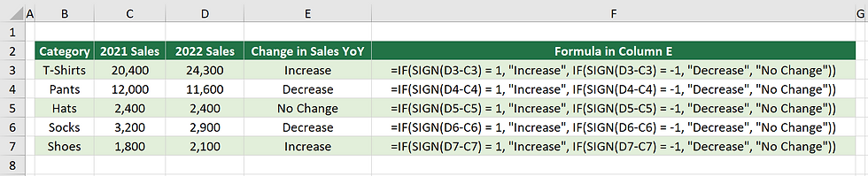
4. Combining the SIGN function and Conditional Formatting to Track Increases and Decreases
Similar to the example above, we will be using the 1, 0, -1 returns from the SIGN formula to give us a visual indication of how sales have moved year over year.
In column E, we are just using the below formula to return a 1 for any increase, -1 for a decrease, and 0 if there was no change.
= SIGN(D3-C3)But, we'll also want to use conditional formatting, to give our report some color and easily let anyone see sales movement at a glance.
To do that, select the cells containing the SIGN formula, and on the ribbon "Home Tab", navigate to conditional formatting > Icon Sets > and select the one that fits your data the best. Here we used the 2nd colored direction one.

You'll end up with results that look like this. Very clean and easy to see how your sales are performing year over year.